Bayesian model evaluation and comparison
Suppose you have a Bayesian statistical model. How do you know it’s a good one? How do you know it isn’t fundamentally misspecified? How do you compare it to alternative model specifications? This post covers the material I’m studying for my comprehensive exam around Bayesian model evaluation (and checking and comparison).
But beyond studying for comps, this material has inspired some thoughts related to topic modeling. Most probabilistic topic models are Bayesian. The core topic of my research is about building better topic models more consistently. I wonder about the degree to which these methods would apply (meaningfully) to topic modeling. Food for thought…
For the below, I use the following convetions:
- \(X\) is the data
- \(\theta\) is the parameter (or parameters) being estimated
- \(\mathcal{L}()\) is the likelihood function
- \(\mathcal{l}()\) is the log of \(\mathcal{L}()\)
- \(B\) is the number of samples drawn in a Markov chain
Checking convergence
Most Bayesian models are fit using some sort of MCMC sampling. I won’t get into the details in this post. However, like backpropagation and other methods, MCMC is is iterative. It iteratively samples from the posterior and then updates estimates based on what’s sampled. This means that we need to ensure that the model has stabilized, or converged. Convergence is when the \(j\)-th sample is independent of the \(j-b\)-th samples. To do this, one generally discards the initial iterations (which we know will not be independent). If your model has not converged, then there’s no point in doing any other evaluation, diagnostics, inference, etc. because you wouldn’t be able to differentiate between a poor evaluation due to model misspecification or because your model didn’t converge, for example.
Convergence is assessed on the last B iterations. Typically convergence is assessed against the parameters being estimated. However, for models like LDA (and other topic models), there are so many parameters, that checking them all is infeasible for both computational and storage reasons. In this case, we typically assess convergence on an overall statistic, like the log likelihood.
The convergence methods I’ll cover here are:
- Geweke’s convergence statistic
- Gelmen-Rubin convergence statistic
- Autocorrelation function plots
Geweke convergence statistic
The Geweke convergence statistic is fairly straightforward.
- Take two non-overlapping (and ordered) subsets of samples from your chain. (e.g. Take the first 10% vs. the last 50% of the chain.)
- Calculate the mean over each subset.
- Perform a difference in means test.
If the chain is stationary (i.e. if the model has converged) the means won’t be different.
One change here is that you have to use autocorrelation consistent standard error.
In the R function coda::geweke.stat, the documentation states that “[t]he standard error is estimated from the spectral density at zero and so takes into account any autocorrelation.”
Gelmen-Rubin statistic
This statistic is a bit more complicated. The bottom line is that you calculate a statistic called a “scale reduction factor”, \(\hat{R}\), that must be less than 1.2 to show convergence. Unlike the Geweke stat., you have to run more than one chain to calculate the Gelmen-Rubin statistic.
The procedure is as follows:
- Run \(m \geq 2\) chains of length \(b = 2n\).
- Discard the first 50% (or first \(n\)) samples from each chain.
- Calculate the average within chain variance, \(W = \frac{1}{m}\sum_{j = 1}^m s^2_j\) where \(s^2_j = \frac{1}{n - 1}\sum_{i=1}^n (\theta_{i,j} - \bar\theta_j)^2\).
- Calculate the between chain variance, \(B = \frac{n}{m - 1}\sum_{j=1}^m(\bar\theta_j - \bar{\bar\theta})\) where \(\bar{\bar\theta} = \frac{1}{m}\sum_{j = 1}^m \bar\theta_j\).
- Calculate the variance of \(\hat\theta\) as a combination of within chain and between chain variance, \(\text{var}(\hat\theta) = \left(1 - \frac{1}{n}\right)W + \frac{1}{n}B\).
- Calculate the scale reduction factor, \(\hat{R} = \sqrt{\frac{\text{var}(\hat\theta)}{W}}\).
- If \(\hat{R} \leq 1.2\) then your chains have converged.
Autocorrelation function plot
This isn’t a convergence statistic per-se. Rather, it displays how correlated (on average) a sample is to the \(k\) samples preceeding it. If a sample is corrlated with preceeding samples, then it’s unlikely that the samples are independent.
I won’t get into the math. (TBH, I don’t expect to get tested on it.) But below is some R code that demonstrates the ACF plot of an independent sample and a sample that is very much not independent. In general, we want the correlations to be close to zero to show independence (and thus chain convergence).
First, generate a chain of independent samples, x_ind and a chain where the current sample depends on the previous sample, x_dep.
# generate an independent sample
x_ind <- rnorm(n = 1000, mean = 0, sd = 1)

# generate a sample whose current value depends on preceeding values
x_dep <- numeric(1000)

x_dep[1] <- rnorm(1, 0, 1)

for (j in seq_along(x_dep)[-1]) {

  x_dep[j] <- rnorm(1, mean = x_dep[j - 1], sd = 1)

}
Now plot the independent ACF.
acf(x_ind, main = "ACF of chain of independent samples")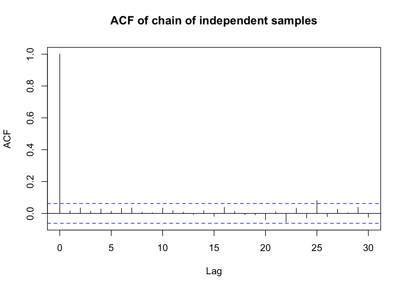
And the non-independent ACF.
acf(x_dep, main = "ACF of chain of non-independent samples")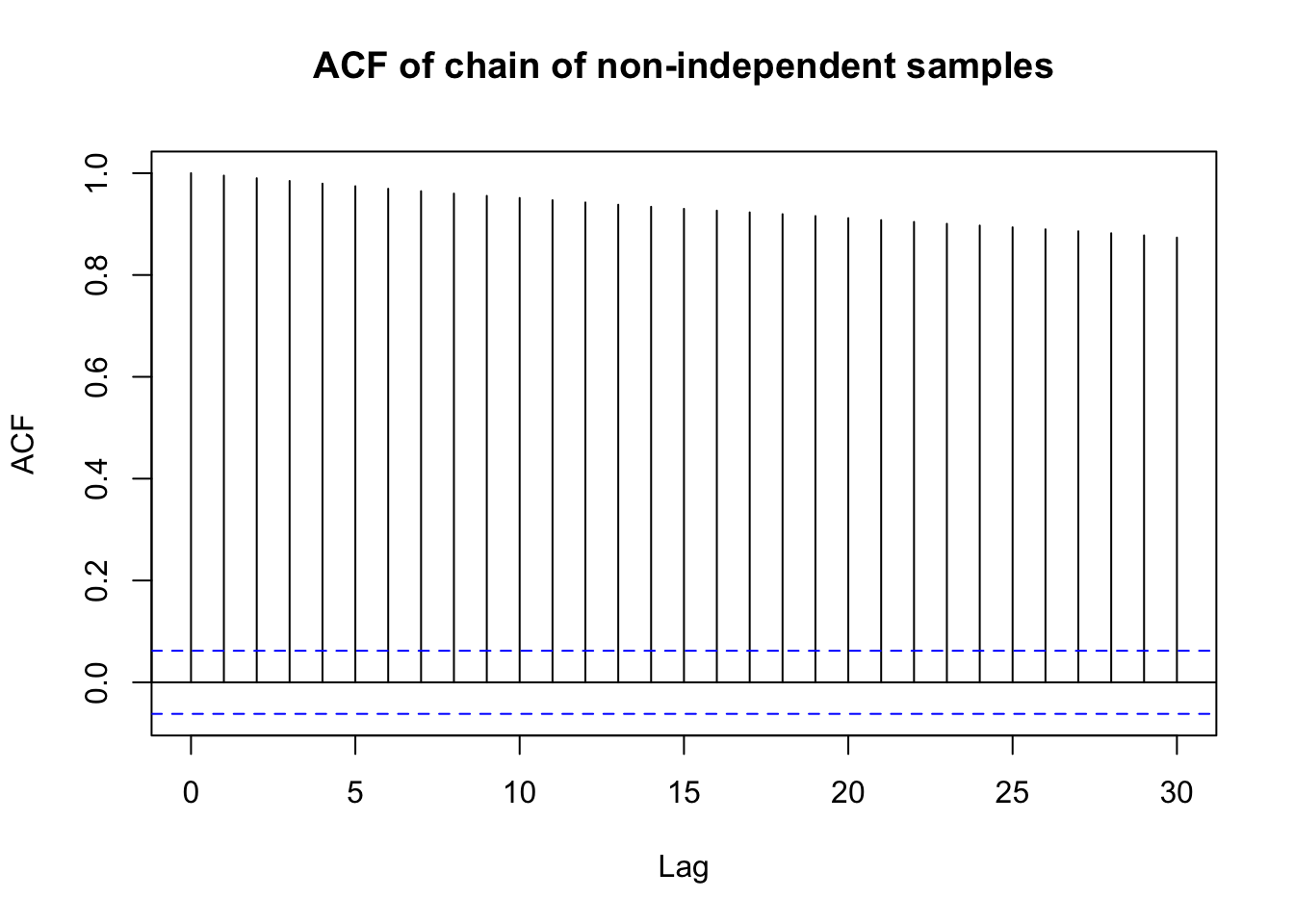
Checking for misspecification
Misspecification evaluations check whether or not your model has poor properties. If it does, maybe you need different prior parameters. Maybe you need a different prior distribution. Maybe you need a different likelihood distribution. Of course, even if everything looks good, there’s no guarantee that your model still isn’t pathologically misspecified. Caveat emptor!
The methods discussed below are:
- Sensitivity analysis
- Mixture model approach
- External validation
- Posterior predictive check
Sensitivity analysis
A sensitivity analysis examines how the posterior distribution changes based on changes to the model specification. This may include changes in:
- The prior parameters
- The prior distribution
- The likelihood distribution
Mixture model approach
When you have many different models (combinations of likelihoods and priors) that you think might be valid. One strategy might be to combine them into an “exhaustive probability model”. Here, your posterior, \(P(\theta|X, \text{etc.})\), is a linear combination of all the models you think might be valid. Then you can perform a sensitivity analysis on the total posterior by tweaking elements of each individual input.
For each likelihood \(\mathcal{L}_j\) and prior \(\pi_j\) the posterior is
\[\begin{align} P(\theta|X, \text{other params.}) &\propto \lambda_1\mathcal{L}_1\pi_1 + \lambda_2\mathcal{L}_2\pi_2 + \lambda_3\mathcal{L}_3\pi_3 + ... \end{align}\]
where \(\sum_j \lambda_j = 1\).
External validation
For those familiar with machine learning, this should be familiar. How well does your Bayesian model predict held out data? If it is a poor predictor, it is likely not well-specified. Done.
Posterior predictive check
Bayesian models are generative. A posterior predictive check has you sampling from the posterior. Then take your posterior samples and compare them to your data. (My reference doesn’t specify training data or held out data. Why not do both?)
Tail area probabilities
You can use a test statistic to compare the posterior samples with the observed data. For example, do they have different means and standard deviations? Maybe you can do a chi-squared test for equality of distribution.
To make this Bayesian, draw many samples and calculate many test statistics. You then get a distribution of statistics and can accept or reject a null hypothesis based on that.
Comparing models
Sometimes you have two models. Maybe they were fit on the same data. Maybe they weren’t. But the bottom line is, you want to know which one is better. In frequentist statistics, one often uses the Akaike information criterion or AIC. There are two information criterion that may be used for Bayesian models. There is also the concept of a Bayes factor, which calculates support for one model over another.
Topics discussed here are:
- Deviance information criterion (DIC)
- Wantanabe Akaike information criterion (WAIC)
- Bayes factors
Deviance information criterion
Like AIC, DIC is negative and smaller values are better. It’s kind of Bayesian in that it’s calculated across samples in the chain. However it’s not fully Bayesian in that it conditions on a point estimate, \(\hat\theta\). (\(\hat\theta\) may be an average over part of your Markov chain or it might be the parameter estimate on the last iteration.) You can calculate it by
\[\begin{align} DIC &= -2 \log \left(\mathcal{L}(X|\hat\theta)\right) + 2 P_{DIC}\\ \text{where}&\\ P_{DIC} &= 2\left(\mathcal{l}(X|\theta) - \frac{1}{B}\sum_{b = 1}^B\mathcal{l}(X|\theta^{(b)})\right)\\ &= 2 \text{var}(\mathcal{l}(X|\theta)) \end{align}\]
where \(\mathcal{l}()\) is the log likelihood function and \(B\) is the number of samples.
Wantanabe Akaike information criterion
WAIC is like AIC and DIC in that smaller is better. WAIC has the advantage of averaging over the posterior distribution rather than conditioning on a point estimate. You can caluclate it by
\[\begin{align} WAIC &= -2\text{lppd} + 2P_{WAIC}\\ &\text{where}\\ \text{lppd} &= \sum_{i = 1}^n \log\left( \frac{1}{B}\sum_{b=1}^B \mathcal{L}(X|\theta^{(b)}\right)\\ &\text{and}\\ P_{WAIC} &= \sum_{i=1}^n \frac{1}{B-1}\sum_{b=1}^B \left( \mathcal{l}(X_i|\theta^{(b)}) - \frac{1}{B}\sum_{b=1}^B \mathcal{l}(X_i|\theta^{(b)}\right)^2 \end{align}\]
Bayes Factors
Bayes factors give you evidence for one model over another, specifically one posterior over another. i.e. for \(H_2\) over \(H_1\), calculate\(\frac{P(H_2|X)}{P(H_1|X)} = \frac{H_2}{H_1}\times \text{BF}(H_2;H_1)\). The goal when using Bayes Factors is to choose a single model \(H_i\) or average over a discrete set using their posterior probabilities. Bayes factors work well when the underlying model is truly discrete.
The Bayes factor of \(H_2\) over \(H_1\) is
\[\begin{align} \text{BF}(H_2;H_1) &= \frac{P(X|H_2)}{P(X|H_1)}\\ &= \frac{\int P(\theta_2,X|H_2)d\theta_2}{\int P(\theta_1,X|H_1)d\theta_1} \end{align}\]
You can interpret the Bayes factor using the following:
| \(\textbf{BF}\boldsymbol{(H_2;H_1)}\) | Interpretation |
|---|---|
| \(< 1\) | Supports \(H_1\) |
| \(1 - 3.2\) | Approximate evidence for \(H_1\) and \(H_2\) are the same |
| \(3.2 - 10\) | Substantial support for \(H_2\) |
| \(10 - 31.6\) | Strong support for \(H_2\) |
| \(31.6 - 100\) | Very strong support for \(H_2\) |
| \(> 100\) | Decisive support for \(H_2\) |
Bayes factors aren’t just a model comparison. They’re a type of Bayesian inference since you are using the posteriors of two models to find evidence supporting one over the other.
Tommy Jones
I like answering boring statistical questions about exciting machine learning models.